Estimating the value of π using a Monte Carlo simulation.
- Emanuel Hoque

- May 12, 2020
- 3 min read
A little history about Monte Carlo simulation: The concept was invented by the Polish American mathematician, Stanislaw Ulam. Probably more well known for his work on thermonuclear weapons than on mathematics. The story goes as: he was ill, recovering from some serious illness, and got a bad habit of playing a lot of solitaire, a game I suspect you've all played. Being a mathematician, he naturally wondered, what's the probability of his winning this stupid game, anyway? After spending a lot of time trying to estimate them by pure combinatoric calculations, he wondered whether a more practical method than "abstract thinking" might not be to lay it out say one hundred times and simply observe and count the number of successful plays. Well, obviously he didn't; rather asked John von Neumann, who is often viewed as the inventor of the stored program computer "Could you do this on your fancy new ENIAC machine?" Well that simulation at that times must have taken hours, which is microseconds in our computational time.
The simulation that I programmed will randomly throw darts (well, obviously not physically) and count the number of hits.
We take a population of the universal set of certain example and a proper subset and then we make an inference about the population based upon some set of statistics, we do on the sample. So the population is typically a very large set of examples, and the sample is a smaller set of examples. In our case the population of incredibly large number of throws indicates the universal set and the number of hits signifies the proper subset.
from random import random
from math import pow, sqrt
darts = 1000000
hits = 0
throws = 0
for i in range (1, darts):
throws += 1
x = random()
y = random()
dist = sqrt(pow(x, 2) + pow(y, 2))
if dist <= 1.0:
hits = hits + 1.0
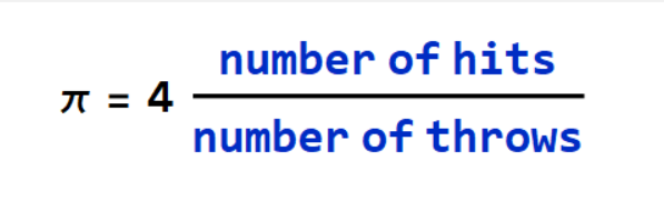
pi = 4*(hits/throws)
print("pi = ", pi)
OUTPUT:
pi =  3.146161514055151
>>>
The key fact that makes them work is that if we choose the sample at random, the sample will tend to exhibit the same properties as the population(that has been tried for a large number of times) from which it is drawn, keeping in mind that the probabilistic chance of any sample occurring is independent of any other sample occurring.
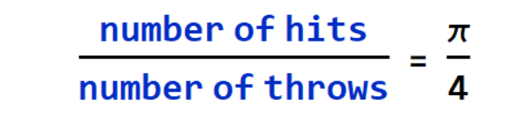
The probability of single hit is given by,

Now, a single throw(sample) exhibit this probability and hence will be reflected as the nature of the population for large number of trials of the sample; that gives:
In simple example, try tossing a coin for a incredibly large number of times. The number of heads (or tails) will keep approaching to be exactly half of the number of tosses i.e. the odds of occurring head (or tail) in a single toss.
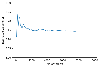
Well the approximated value isn't quite precise, considering the fact that 10 to the power 6 trials, approximated it. Let us check the trend from a lower number to a higher number of throws. I stored a few of number of throws from 100 to 10000 and their corresponding approximated value of π and plotted the trend.
from random import random
from math import pow, sqrt
import matplotlib.pyplot as plt

hits = 0
throwCount = 0
darts = []
valuesPi = []

for throws in range(100,10000,100):
    darts.append(throws)
    for i in range (1, throws):
        throwCount += 1
        x = random()
        y = random()
        dist = sqrt(pow(x, 2) + pow(y, 2))
        if dist <= 1.0:
            hits += 1.0
    valuePi = 4*(hits/throwCount)
    valuesPi.append(valuePi)

plt.plot(darts,valuesPi)
plt.xlabel("No of throws")
plt.ylabel("Estimated value of pi")
plt.ylim(3.00,3.30)
plt.show()


Comments