Numerical Integration using Monte Carlo method (the naive approach).
- Emanuel Hoque

- May 13, 2020
- 2 min read
There's two approach of numerical integration: deterministic and non-deterministic. Monte Carlo's method of integration employs non-deterministic approach, since random numbers are at play. In simple words, every manipulation yields different results. The magical thing about Monte Carlo method of integration is that, it corresponds to a normal distribution (as in the case of any Monte Carlo Simulation) about the exact value of integration and hence the error bars are known. What exactly, is approach then?
Monte Carlo method of integration generally addresses multivariable definite integral.

where Ω, a subset of Rm, has volume,

The naive Monte Carlo approach is to sample points uniformly on Ω: given N uniform samples,

The value of integration can be approximated as,

and the law of large numbers ensures that as limit N tends to infinity, the exact value is approximated.
Given, the estimation of I, error bars can be estimated by the sample variance using the unbiased estimate of the variance.

where,

Why not, validate it by actually doing an integration.
import random
import numpy as np
import matplotlib.pyplot as plt

aX = 0
aY = np.pi
bX = np.pi
bY = 2*np.pi
N = 10000
n = 1000
x = []
integrals = []

def f(x, y):
    return np.sin(x*y)

for i in range(n):
    sumf = 0
    for i in range(N):
        xi = random.uniform(aX, bX)
        yi = random.uniform(aY, bY)
        sumf += f(xi, yi)
    integral = ((bX-aX)*(bY-aY)*sumf)/N
    integrals.append(integral)

plt.title("Distribution of the integrals")
plt.hist(integrals,bins=40)
plt.xlabel("Integrals")
plt.show()

avgIntegral = sum(integrals)/len(integrals)
print("The value of integration is ",avgIntegral)
Here is a code for integrating sin(x*y) from x: 0 to π and y: π to 2π. It samples 10,000 random values of x between 0 to π and 10,000 random values of y between π to 2π, then finds the value of the function f(x,y) = sin(x*y) for those random 10,000 values of x and y and the gradually adding those values of the function. To find the integral, we multiply it by lengths of the limits for x and y and dividing it by number of samples. In a simple notion, it is like finding volume of a lot of cuboids whose length corresponds to length of limits of x and breath to that of length of limits of y and height corresponding to the point (xi, yi) for different random samples, some under the curve and some above. The law of large numbers takes care of the fact that if the sample numbers of these cuboids are very large, the volume under the curve f(x,y) can be approximated.
We are not done yet. We know for a fact that every different simulation will yield different value and the distribution of those samples will be a normal distribution about the exact value of integration. Hence if we find the average of these samples, we yield more accurate value even for low sampling of random values of (x, y). I also plotted an histogram with 40 bins to visualise the distribution.
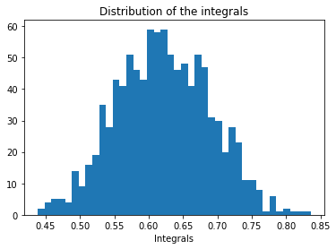
The value of integration is 0.621715880705006


Comments